45 excel chart custom data labels
Make your Excel charts easier to read with custom data labels Click the Chart Wizard button in the standard tool bar. Click Line under Chart Type. Click Next twice. In the Chart Title box, enter 2006 Region One Sales. Click the Legend tab, and clear the Show... How do I put custom data labels on charts in Excel? I have a chart showing burn rates (fairly small numbers) and EACs/ETCs(Relly big numbers). I have set up 2 Y-Axis, but this stretches the burn rate a lot, so if it changes a little bit, it adjusts the axis and suddenly, a 1% spike goes all the way from the bottom edge to the top. I know I can define the axis to compensate, but then if there really were a spike, it has the potential to go off ...
How to Make a Pie Chart in Excel & Add Rich Data Labels to ... Sep 08, 2022 · In this article, we are going to see a detailed description of how to make a pie chart in excel. One can easily create a pie chart and add rich data labels, to one’s pie chart in Excel. So, let’s see how to effectively use a pie chart and add rich data labels to your chart, in order to present data, using a simple tennis related example.
Excel chart custom data labels
Change the format of data labels in a chart To get there, after adding your data labels, select the data label to format, and then click Chart Elements > Data Labels > More Options. To go to the appropriate area, click one of the four icons ( Fill & Line, Effects, Size & Properties ( Layout & Properties in Outlook or Word), or Label Options) shown here. How to add text labels on Excel scatter chart axis - Data Cornering Add dummy series to the scatter plot and add data labels. 4. Select recently added labels and press Ctrl + 1 to edit them. Add custom data labels from the column "X axis labels". Use "Values from Cells" like in this other post and remove values related to the actual dummy series. Change the label position below data points. Custom Chart Data Labels In Excel With Formulas - How To Excel At Excel Follow the steps below to create the custom data labels. Select the chart label you want to change. In the formula-bar hit = (equals), select the cell reference containing your chart label's data. In this case, the first label is in cell E2. Finally, repeat for all your chart laebls.
Excel chart custom data labels. Custom Excel Chart Label Positions • My Online Training Hub Custom Excel Chart Label Positions Watch on Download Workbook Get Workbook Custom Excel Chart Label Positions - Setup The source data table has an extra column for the 'Label' which calculates the maximum of the Actual and Target: Excel tutorial: How to customize axis labels Now let's customize the actual labels. Let's say we want to label these batches using the letters A though F. You won't find controls for overwriting text labels in the Format Task pane. Instead you'll need to open up the Select Data window. Here you'll see the horizontal axis labels listed on the right. Click the edit button to access the ... How to Change Excel Chart Data Labels to Custom Values? May 05, 2010 · Now, click on any data label. This will select “all” data labels. Now click once again. At this point excel will select only one data label. Go to Formula bar, press = and point to the cell where the data label for that chart data point is defined. Repeat the process for all other data labels, one after another. See the screencast. Add data labels and callouts to charts in Excel 365 - EasyTweaks.com Step #1: After generating the chart in Excel, right-click anywhere within the chart and select Add labels . Note that you can also select the very handy option of Adding data Callouts. Step #2: When you select the "Add Labels" option, all the different portions of the chart will automatically take on the corresponding values in the table ...
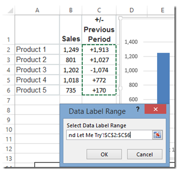
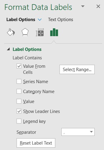
Excel Custom Data Labels with Symbols that change ... - YouTube May 7, 2020 ... In this tutorial we will learn how to format Data labels in Excel Charts to make them dynamically change their colors. Using the CONCAT function to create custom data labels for an Excel chart Use the chart skittle (the "+" sign to the right of the chart) to select Data Labels and select More Options to display the Data Labels task pane. Check the Value From Cells checkbox and select the cells containing the custom labels, cells C5 to C16 in this example. How to Use Cell Values for Excel Chart Labels - How-To Geek Select the chart, choose the "Chart Elements" option, click the "Data Labels" arrow, and then "More Options." Uncheck the "Value" box and check the "Value From Cells" box. Select cells C2:C6 to use for the data label range and then click the "OK" button. The values from these cells are now used for the chart data labels. Create Dynamic Chart Data Labels with Slicers - Excel Campus Step 6: Setup the Pivot Table and Slicer. The final step is to make the data labels interactive. We do this with a pivot table and slicer. The source data for the pivot table is the Table on the left side in the image below. This table contains the three options for the different data labels.
Present data in a chart - support.microsoft.com In addition to applying a predefined chart style, you can easily apply formatting to individual chart elements such as data markers, the chart area, the plot area, and the numbers and text in titles and labels to give your chart a custom, eye-catching look. How to Customize Your Excel Pivot Chart Data Labels - dummies The Data Labels command on the Design tab's Add Chart Element menu in Excel allows you to label data markers with values from your pivot table. When you click the command button, Excel displays a menu with commands corresponding to locations for the data labels: None, Center, Left, Right, Above, and Below. None signifies that no data labels ... Custom data labels in a chart - Get Digital Help Add data labels Press with right mouse button on on a column Press with left mouse button on "Add Data Labels" Double press with left mouse button on a data label Deselect Value Select Category name Press with left mouse button on Close Get the Excel file Custom-data-labels-in-a-chartv3.xlsx Charts category Add pictures to a chart axis Actual vs Budget or Target Chart in Excel - Variance on ... Aug 19, 2013 · Set Data Labels to Cell Values Screenshot Excel 2003-2010. The nice part about either of these methods is that the data labels are linked to the values in the cells. If your numbers change or you update the data, the labels will automatically be refreshed and display the correct results. Please let me know if you have any questions.
Help Online - Quick Help - FAQ-133 How do I label the data ...
How to add data labels from different column in an Excel chart? Right click the data series in the chart, and select Add Data Labels > Add Data Labels from the context menu to add data labels. 2. Click any data label to select all data labels, and then click the specified data label to select it only in the chart. 3.
How to Customize Your Excel Pivot Chart and Axis Titles - dummies
Create Custom Data Labels. Excel Charting. - YouTube Jan 23, 2022 ... Are you looking to create custom data labels to your Excel chart? Maybe you want to add the title of a song or the name of a magazine.

how to add data labels into Excel graphs — storytelling with data
Add Custom Labels to x-y Scatter plot in Excel Step 1: Select the Data, INSERT -> Recommended Charts -> Scatter chart (3 rd chart will be scatter chart) Let the plotted scatter chart be. Step 2: Click the + symbol and add data labels by clicking it as shown below. Step 3: Now we need to add the flavor names to the label. Now right click on the label and click format data labels.
Custom Data Labels - Microsoft Power BI Community
Excel Custom Chart Labels • My Online Training Hub Note: Excel 2013 onward also requires this step if you have more than one series you want to position your labels above. Step 1: Select cells A26:D38 and insert a column Chart. Step 2: Select the Max series and plot it on the Secondary Axis: double click the Max series > Format Data Series > Secondary Axis: Step 3: Insert labels on the Max ...
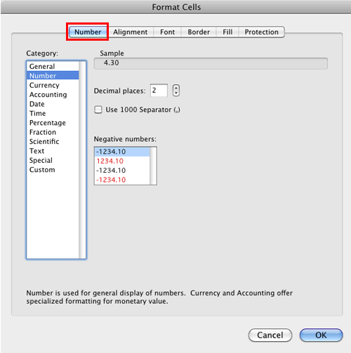
Format Number Options for Chart Data Labels in Excel 2011 for Mac
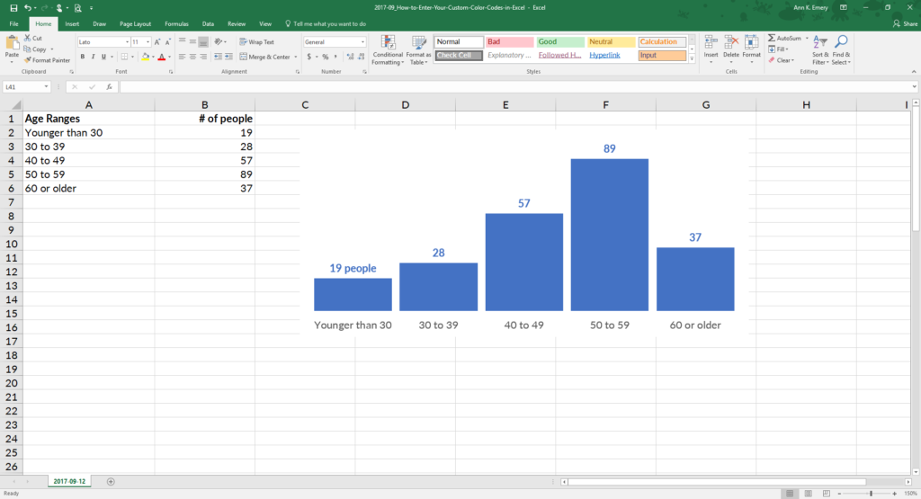
Custom Data Labels with Colors and Symbols in Excel Charts - [How To ... The basic idea behind custom label is to connect each data label to certain cell in the Excel worksheet and so whatever goes in that cell will appear on the chart as data label. So once a data label is connected to a cell, we apply custom number formatting on the cell and the results will show up on chart also.

How-to Use Data Labels from a Range in an Excel Chart - Excel ...
How to add and customize chart data labels - Get Digital Help Edit data labels. Excel allows you to edit the data label value manually, simply press with left mouse button on a data label until it is selected. Press with left mouse button on again to select the text, you can now type any value you want. I changed the data label value to "Look here!". You can link a group of data labels to a cell range so ...
How-to Use Data Labels from a Range in an Excel Chart - Excel ...
How to Adjust Your Bar Chart’s Spacing in Microsoft Excel Jun 02, 2015 · In a line chart or a stacked line chart (a.k.a. stacked area chart), you can move the categories closer together by narrowing the graph. By default, Excel graphs are 3 inches tall and 5 inches wide. To nudge the categories closer together, you would adjust your graph so that it’s, let’s say, 3 inches tall and 4 inches wide.
Directly Labeling Excel Charts - PolicyViz
How to create Custom Data Labels in Excel Charts - Efficiency 365 Create the chart as usual Add default data labels Click on each unwanted label (using slow double click) and delete it Select each item where you want the custom label one at a time Press F2 to move focus to the Formula editing box Type the equal to sign Now click on the cell which contains the appropriate label Press ENTER That's it.
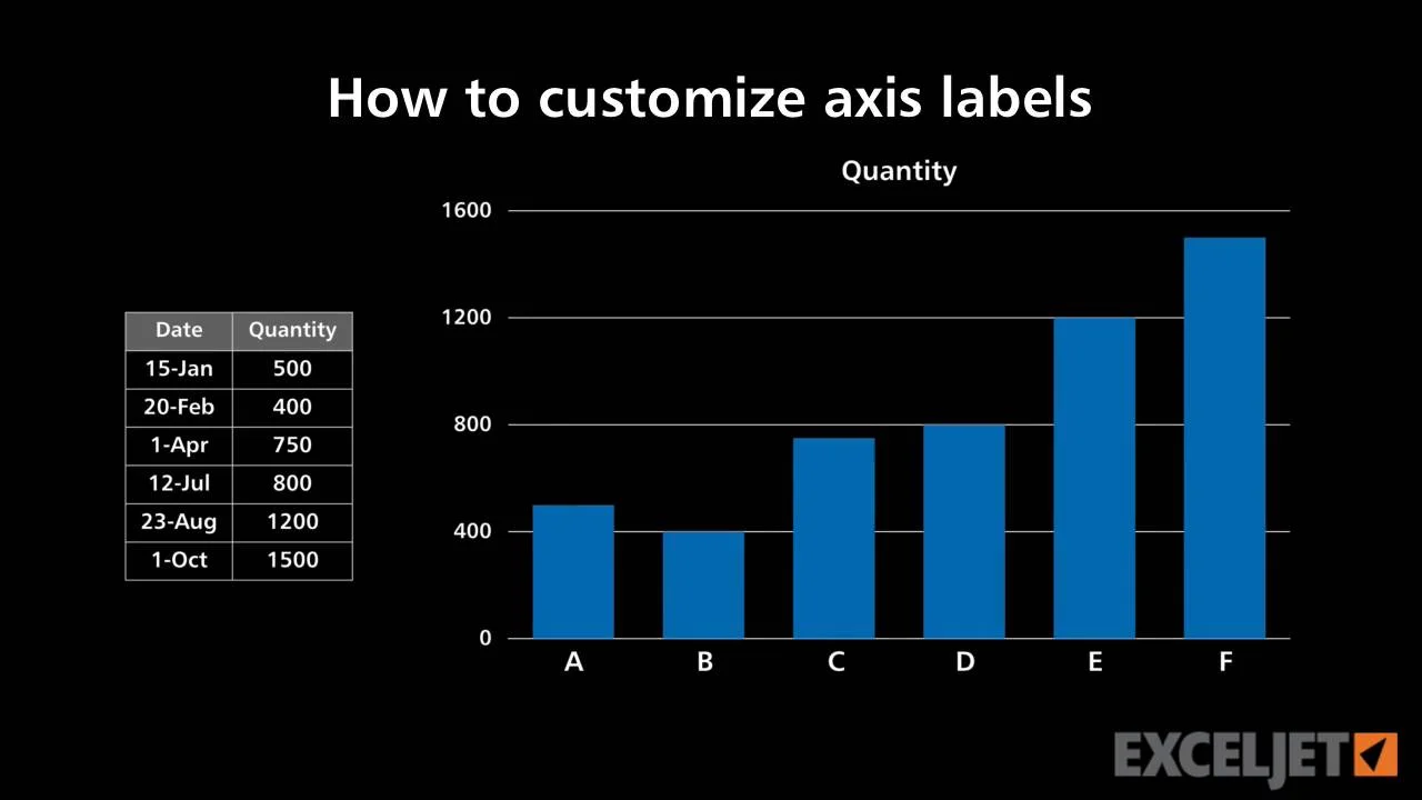
How to customize axis labels
Xlsxwriter Excel Chart Custom Data Label Position At default the custom labels seem to bet set at right. I want them on top but I cant get this. The code is like that: chart.add_series ( .., 'data_labels': {'custom': my_custom_labels, 'position': 'above'}) But the changes wont appy to the chart. I also found i can set the default label position (label_position_default) in the chart object ...

Change axis labels in a chart
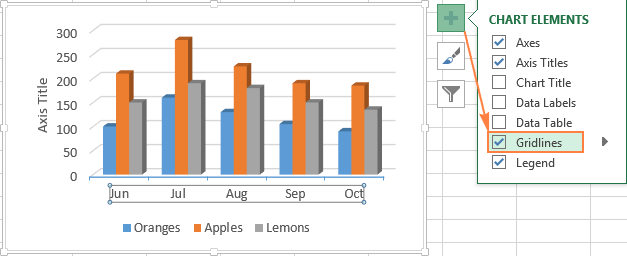
Excel charts: add title, customize chart axis, legend and data labels Click the Chart Elements button, and select the Data Labels option. For example, this is how we can add labels to one of the data series in our Excel chart: For specific chart types, such as pie chart, you can also choose the labels location. For this, click the arrow next to Data Labels, and choose the option you want.

Adding rich data labels to charts in Excel 2013 | Microsoft ...
Add / Move Data Labels in Charts - Excel & Google Sheets Double Click Chart Select Customize under Chart Editor Select Series 4. Check Data Labels 5. Select which Position to move the data labels in comparison to the bars. Final Graph with Google Sheets After moving the dataset to the center, you can see the final graph has the data labels where we want.

Change color of data label placed, using the 'best fit ...
[Solved] Charts: custom data labels - Excel General - OzGrid Free Excel ... I have a pivot table with Due Date and Library Name as row headings and % Finished as data. I'd like to chart the table so that the X-axis is Library Name, the height of the bar is %Finished and the data label is Due Date. I don't have to use a pivot table for this. A normal table with 3 columns would be fine. ie Library,Value,Label
Excel Charts: Creating Custom Data Labels
Example: Charts with Data Labels — XlsxWriter Documentation Chart 1 in the following example is a chart with standard data labels: Chart 6 is a chart with custom data labels referenced from worksheet cells: Chart 7 is a chart with a mix of custom and default labels. The None items will get the default value. We also set a font for the custom items as an extra example: Chart 8 is a chart with some ...

Data Labels in Power BI - SPGuides
Apply Custom Data Labels to Charted Points - Peltier Tech There are a number of ways to apply custom data labels to your chart: Manually Type Desired Text for Each Label Manually Link Each Label to Cell with Desired Text Use the Chart Labeler Program Use Values from Cells (Excel 2013 and later) Write Your Own VBA Routines Manually Type Desired Text for Each Label
How to Enter Your Custom Color Codes in Microsoft Excel ...
Excel Charts: Creating Custom Data Labels - YouTube Excel Charts: Creating Custom Data Labels 91,765 views Jun 26, 2016 210 Dislike Share Save Mike Thomas 4.58K subscribers In this video I'll show you how to add data labels to a chart in Excel and...

Change the format of data labels in a chart
Add or remove data labels in a chart - support.microsoft.com Click the data series or chart. To label one data point, after clicking the series, click that data point. In the upper right corner, next to the chart, click Add Chart Element > Data Labels. To change the location, click the arrow, and choose an option. If you want to show your data label inside a text bubble shape, click Data Callout.

Color Negative Chart Data Labels in Red with downward arrow
How to Create a SPEEDOMETER Chart [Gauge] in Excel Now, select the data labels and open “Format Data Label” and after that click on “Values from Cells”. From here, select the performance label from the first data table and then untick “Values”. After that, select the label chart and do the same with it by adding labels from the second data table. And at last, you need to add a ...

Apply Custom Data Labels to Charted Points - Peltier Tech
Custom Chart Data Labels In Excel With Formulas - How To Excel At Excel Follow the steps below to create the custom data labels. Select the chart label you want to change. In the formula-bar hit = (equals), select the cell reference containing your chart label's data. In this case, the first label is in cell E2. Finally, repeat for all your chart laebls.

How to Add Custom Data Labels at Specific Position in Chart JS
How to add text labels on Excel scatter chart axis - Data Cornering Add dummy series to the scatter plot and add data labels. 4. Select recently added labels and press Ctrl + 1 to edit them. Add custom data labels from the column "X axis labels". Use "Values from Cells" like in this other post and remove values related to the actual dummy series. Change the label position below data points.

How to format axis labels individually in Excel
Change the format of data labels in a chart To get there, after adding your data labels, select the data label to format, and then click Chart Elements > Data Labels > More Options. To go to the appropriate area, click one of the four icons ( Fill & Line, Effects, Size & Properties ( Layout & Properties in Outlook or Word), or Label Options) shown here.

Custom Data Labels with Colors and Symbols in Excel Charts ...

Excel Charts - Aesthetic Data Labels

Display Customized Data Labels on Charts & Graphs

Data Labels in FlexChart | Features | Wijmo Docs

How to Customize for a GREAT-Looking Excel Chart

Improve your X Y Scatter Chart with custom data labels

excel - How to show series-Legend label name in data labels ...

Google Workspace Updates: Get more control over chart data ...
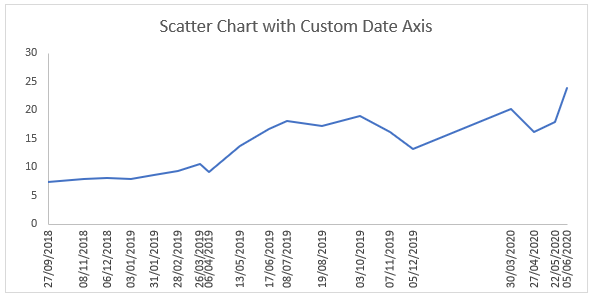
Label Specific Excel Chart Axis Dates • My Online Training Hub

Custom Excel Chart Label Positions • My Online Training Hub

Add Custom Labels to x-y Scatter plot in Excel - DataScience ...
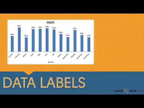
Adding Data Labels To An Excel Chart | MyExcelOnline
Custom Y-Axis Labels in Excel - PolicyViz

Change Horizontal Axis Values in Excel 2016 - AbsentData

Google Workspace Updates: New chart text and number ...
Using the CONCAT function to create custom data labels for an ...

How to set and format data labels for Excel charts in C#

Adding rich data labels to charts in Excel 2013 | Microsoft ...

Adding rich data labels to charts in Excel 2013 | Microsoft ...
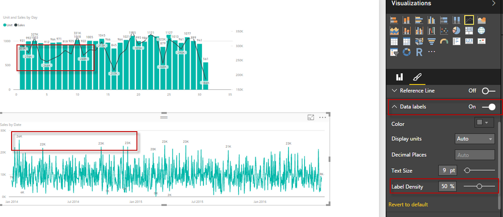
Solved: Data Labels - Microsoft Power BI Community
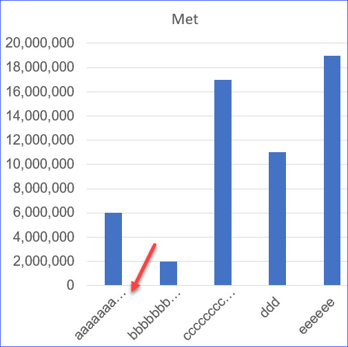
How to Wrap X Axis Labels in an Excel Chart - ExcelNotes
Excel charts: add title, customize chart axis, legend and ...
Excel axis labels - supercategory — storytelling with data

Custom Data Labels with Colors and Symbols in Excel Charts ...

Solved: How to show all detailed data labels of pie chart ...
Post a Comment for "45 excel chart custom data labels"